4. O&M
Observations & Measurements
In addition to the definition of relevant terms within the SWE framework presented above, a more detailed explanation of how an observation is modeled is presented subsequently. The information is a summary of the official OGC Observations & Measurements standard version 2.0, which can be downloaded from
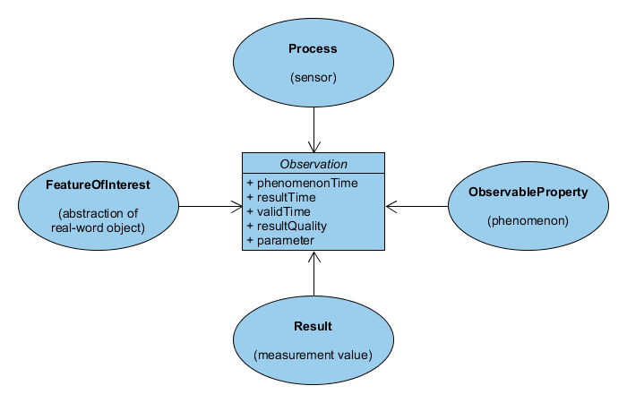
The following figure presents an overview of the components of an observation (Bröring et al. 2011 a). Note that the figure has been simplified in order to omit complex information.

An observation is a composed object providing relevant observation details. In consequence, an observation belongs to a procedure that measured a certain observedProperty at a dedicated featureOfInterest for a certain phenomenonTime and stores a result. The property resultQuality indicates the quality of the measured result, as each measurement is faulty to a certain extent by nature.
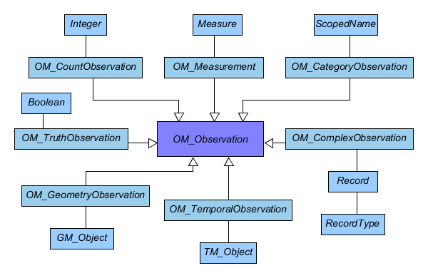
Based on this generic concept, observations are categorized according to their result type. They may be distinguished in discrete and continuous observation. An observation is discrete, when the result represents a spatio-temporal invariant value and applies to the whole area of the referenced featureOfInterest. The possible observation types and their content/result types are illustrated in the below figure. In contrast, a continuous observation measures an observableProperty that may vary in time or for the whole area of a certain featureOfInterest. In that case the result is not represented by a single value, but by a coverage. To model the coverage, distinct sub-geometries are defined to discretise the whole area of the associated feature. In consequence, a single coverage consists of multiple entries, one per sub-geometry and/or timestamp.

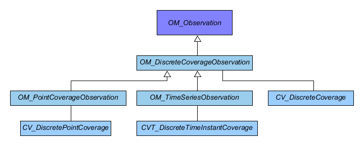
The following figure represents the standardized coverage observation types according to the O&M standard (Cox 2013) in a simplified way. Considering the discretization of an area-based featureOfInterest, the standard introduces two distinct declarations. The whole featureOfInterest as a single object (a spatially distributed entity) is denoted as ultimate feature, whereas each sub-geometry resulting from the discretization process is denoted as a sampling feature. Hence, each concrete measurement value of a coverage observation refers to a sampling feature.

In the following, some examples are given, showcasing encoded O&M documents within certain use cases.
Stationary in-situ Sensors
Stationary in-situ sensors are located at a fixed position directly attached
to the associated featureOfInterest. In consequence, the properties procedure
and featureOfInterest have constant geo-locations and the overall observations
always refer to the same spatial extent (the one of the featureOfInterest). As
an example for stationary in-situ sensors, the below XML illustrates an exemplary
OM_Observation instance of a temperature sensor, measuring
the observedProperty “Ambient temperature”. As result, a simple measurement
value (type OM_Measurement) of the temperature in degree Celcius (parameter
uom of om:result element) is contained. Remarkably, for certain parameters,
only a reference to a named instance is included in the document, e.g. for
the parameters procedure or featureOfInterest. This indicates that more
metadata about those entities can be requested via a dedicated operation of
SWE’s core service, the Sensor Observation Service (more on that later).
<?xml version="1.0" encoding="UTF-8"?>
<om:OM_Observation xmlns:om="http://www.opengis.net/om/2.0" xmlns:gml="http://www.opengis.net/gml/3.2" xmlns:xlink="http://www.w3.org/1999/xlink" gml:id="o_96084693">
   <!-- observation type; here Measurement -->
   <om:type xlink:href="http://www.opengis.net/def/observationType/OGC-OM/2.0/OM_Measurement" />
   <!-- period in time for which the mesaurment applies -->
   <om:phenomenonTime>
      <gml:TimePeriod gml:id="phenomenonTime_96084693">
         <gml:beginPosition>2014-12-30T23:01:00.000Z</gml:beginPosition>
         <gml:endPosition>2014-12-30T23:02:00.000Z</gml:endPosition>
      </gml:TimePeriod>
   </om:phenomenonTime>
   <!-- point in time when the measurement was observed -->
   <om:resultTime>
      <gml:TimeInstant gml:id="ti_14ED5010C900D2F4B0AF30D8C41CF6895C24F539">
         <gml:timePosition>2014-12-30T23:02:00.000Z</gml:timePosition>
      </gml:TimeInstant>
   </om:resultTime>
   <!-- reference to sensor/procedure using its identifier -->
   <om:procedure xlink:href="ENTPE-AmbT-Vaisala-HMP-45AC-QC1" />
   <!-- reference to phenomena using its identifier -->
   <om:observedProperty xlink:href="Ambient Temperature" />
   <!-- reference to featureOfInterest using its identifier -->
   <om:featureOfInterest xlink:href="ENTPE" xlink:title="ENTPE" />
   <!-- result of the observation -->
   <om:result xmlns:ns="http://www.opengis.net/gml/3.2" xmlns:xsi="http://www.w3.org/2001/XMLSchema-instance" uom="degree C" xsi:type="ns:MeasureType">1.1</om:result>
</om:OM_Observation>
Another example of an encoded OM_Measurement observation about solar
irradiance is shown in the below XML. This time, the observedProperty is set
to the phenomenon Direct Horizontal Irradiance and the measured value comprises
"96.0" W per m².
<?xml version="1.0" encoding="UTF-8"?>
<om:OM_Observation xmlns:om="http://www.opengis.net/om/2.0" xmlns:gml="http://www.opengis.net/gml/3.2" xmlns:xlink="http://www.w3.org/1999/xlink" gml:id="o_129748204">
   <!-- observation type; here Measurement -->
   <om:type xlink:href="http://www.opengis.net/def/observationType/OGC-OM/2.0/OM_Measurement" />
   <!-- period in time for which the mesaurment applies -->
   <om:phenomenonTime>
      <gml:TimePeriod gml:id="phenomenonTime_129748204">
         <gml:beginPosition>2014-12-31T09:12:00.000Z</gml:beginPosition>
         <gml:endPosition>2014-12-31T09:13:00.000Z</gml:endPosition>
      </gml:TimePeriod>
   </om:phenomenonTime>
   <!-- point in time when the measurement was observed -->
   <om:resultTime>
      <gml:TimeInstant gml:id="ti_E23CEF5CA8211078069BED5B2D21A72AC1798827">
         <gml:timePosition>2014-12-31T09:13:00.000Z</gml:timePosition>
      </gml:TimeInstant>
   </om:resultTime>
   <!-- reference to sensor/procedure using its identifier -->
   <om:procedure xlink:href="ENTPE-BH-KZ-CH1-QCfull" />
   <!-- reference to phenomena using its identifier -->
   <om:observedProperty xlink:href="Direct Horizontal Irradiance" />
   <!-- reference to featureOfInterest using its identifier -->
   <om:featureOfInterest xlink:href="ENTPE" xlink:title="ENTPE" />
   <!-- result of the observation -->
   <om:result xmlns:ns="http://www.opengis.net/gml/3.2" xmlns:xsi="http://www.w3.org/2001/XMLSchema-instance" uom="W m-2" xsi:type="ns:MeasureType">96.0</om:result>
</om:OM_Observation>
Mobile in-situ sensors
In contrast to a stationary sensor, mobile sensors are not fixed at a
certain geo-location, but vary in space. As a result, the coordinates of
the sensor/procedure may vary for different points in time. Thus, any
associated observation should be modeled as a so-called spatial observation
(type OM_SpatialObservation) according to the Spatial Filtering Profile of the
O&M standard. A spatial observation has to include an additional metadata
parameter carrying the sampling feature/geometry, which indicates the
geo-location of the observation, e.g. any gml:AbstractGeometry such as points,
lines or polygons. A valid parameter definition of a point feature is
illustrated in the below example. Remarkably, the xlink:href attribute value http://www.opengis.net/def/param-name/OGC-OM/2.0/samplingGeometry in the element
om:name denotes the parameter as the sampling feature. The om:value tag
contains a GML point definition.
<om:parameter>
   <om:NamedValue>
      <om:name xlink:href="http://www.opengis.net/def/param-name/OGC-OM/2.0/samplingGeometry" />
      <om:value>
         <gml:Point gml:id="SamplingPoint1">
            <gml:pos srsName="http://www.opengis.net/def/crs/EPSG/0/4326">52.9 7.52</gml:pos>
         </gml:Point>
      </om:value>
   </om:NamedValue>
</om:parameter>
Also note the difference between a single featureOfInterest definition and a sampling feature/geometry. Whereas the featureOfInterest is a static definition of the area of interest, concrete sampling features/geometries denote dynamic spatially varying entities to geo-reference a certain observation within the associated featureOfInterest.
An exemplary observation for a mobile in-situ sensor is discussed within the
context of 52°North enviroCar project (enviroCar 2015). In this citizen
science project, floating car data like fuel consumption, speed or pollution
impact is collected/computed using a dedicated device (OBD II adapter) and
a smartphone app. Via associated analysis functionalities, the data can be
used to optimize driving efficiency and other aspects of sustainable mobility.
As each participating user utilizes his/her smartphone as a GPS-sensor to
geo-reference the acquired car data while driving, this setup can be
denoted as a mobile in-situ sensor. To encode the observation as of type
OM_SpatialObservation, the following mapping definition is recommended:
| O&M Parameter | enviroCar Equivalent |
|---|---|
| Type | OM_SpatialObservation |
| Phenomenon Time | Time instant when performing the measurement |
| Result Time | Time instant when creating/saving the measurement |
| Feature of Interest | No clear definition possible; Within the enviroCar project, multiple measurements are performed/collected for a single track. A track is started by a user when driving around, initiating the systm to frequently perform measurement until the user stops the track. At each measurement, the current GPS position is used as sampling feature (see next table entry). But how can the feature of interest be defined best? An intuitive mapping could be to use the whole geometry of the track (which is a polyline), which is discretized at each concrete measurement location along the path. |
| Parameter Sampling Feature/Geometry | The current (point-based) GPS location of the smartphone when performing the measurement |
| Procedure | OBD II adapter, which is connected to the car |
| Observed Property | One for each car-related phenomenon measured/extracted by the OBD II adapter (e.g. speed, fuel level, ) as well as one for each computed information (such as fuel consumption, estimated fuel cost or CO2 emissions) |
| Result | Stores the measured value according to the observed property |
To illustrate the mapping, an exemplary dataset from the enviroCar project is presented subsequently. Anonymised data can be retrieved using the enviroCar REST API via the link
It provides access to several datasets including tracks, sensors (car definitions), phenomenons (observable properties) and measurements. Of particular relevance is the endpoint
which grants access to concrete measurements. For instance, Figure 8 lists one exemplary measurement encoded in JSON. The key elements with respect to the mapping to O&M are highlighted and annotated (using “comment-style” [sic!]).
{
  "type": "Feature",
  "geometry": { // sampling feature
    "type": "Point",
    "coordinates": [
      6.4847174678758375,
      51.22546715521443
    ]
  },
  "properties": {
    "id": "579634f9e4b086b281bf935e", // observation ID
    "time": "2012-01-01T00:06:44Z", // result/phenomenon time
    "sensor": {
      "type": "car",
      "properties": {
        "engineDisplacement": 2200,
        "model": "Vectra C Caravan",
        "id": "5750591ee4b09078f98673d8", // procedure ID
        "fuelType": "gasoline",
        "constructionYear": 2004,
        "manufacturer": "Opel"
      }
    },
    "track": "579634f9e4b086b281bf935c", // feature of interest ID
    "phenomenons": { // phenomena with results
      "Speed": {
        "value": 0,
        "unit": "km/h"
      },
      "O2 Lambda Voltage ER": {
        "value": 0.9903972702086321,
        "unit": "ratio"
      },
      "Intake Temperature": {
        "value": 29.99999910593033,
        "unit": "c"
      },
      "Consumption": {
        "value": 1.781552855748061,
        "unit": "l/h"
      },
      "O2 Lambda Voltage": {
        "value": 1.452168180985609,
        "unit": "V"
      },
      "MAF": {
        "value": 5.4196322499235805,
        "unit": "l/s"
      },
      "Intake Pressure": {
        "value": 33.99999949336052,
        "unit": "kPa"
      },
      "Engine Load": {
        "value": 20.09168342647675,
        "unit": "%"
      },
      "GPS Accuracy": {
        "value": 8.00000011920929,
        "unit": "%"
      },
      "GPS Speed": {
        "value": 0,
        "unit": "km/h"
      },
      "Rpm": {
        "value": 782.9921875,
        "unit": "u/min"
      },
      "CO2": {
        "value": 4.186649211007944,
        "unit": "kg/h"
      }
    }
  }
}
Each measurement belongs to a certain track, which is referenced by its unique
identifier. A track consists of multiple measurements, each specifying a
concrete position and point in time, where and when the listed phenomena are
observed. Thus, each measurement may be encoded as an OM_SpatialObservation.
For instance, using the phenomenon Consumption, the JSON-encoded observation
might be transformed into O&M as shown in the below example. As suggested the
track identifier is used to reference the featureOfInterest. This mapping
decision however is just within the scope of this document. It is possible
that other definitions of the feature of interest are more applicable.
<?xml version="1.0" encoding="UTF-8"?>
<om:OM_Observation xmlns:om="http://www.opengis.net/om/2.0" xmlns:gml="http://www.opengis.net/gml/3.2" xmlns:xlink="http://www.w3.org/1999/xlink" gml:id="579634f9e4b086b281bf935e">
   <!-- observation type; here SpatialObservation -->
   <om:type xlink:href="http://www.opengis.net/def/observationType/OGC-OM/2.0/OM_SpatialObservation" />
   <!-- period in time for which the mesaurment applies -->
   <om:phenomenonTime>
      <gml:TimeInstant gml:id="/uniqueID/">
         <gml:timePosition>2012-01-01T00:06:44Z</gml:timePosition>
      </gml:TimeInstant>
   </om:phenomenonTime>
   <!-- point in time when the measurement was observed -->
   <om:resultTime>
      <gml:TimeInstant gml:id="/uniqueID/">
         <gml:timePosition>2012-01-01T00:06:44Z</gml:timePosition>
      </gml:TimeInstant>
   </om:resultTime>
   <!-- definition of observation geometry; location where the observation was performed -->
   <om:parameter>
      <om:NamedValue>
         <om:name xlink:href="http://www.opengis.net/def/param-name/OGC-OM/2.0/samplingGeometry" />
         <om:value>
            <gml:Point gml:id="SamplingPoint1">
               <gml:pos srsName="http://www.opengis.net/def/crs/EPSG/0/4326">51.22546715521443, 6.4847174678758375</gml:pos>
            </gml:Point>
         </om:value>
      </om:NamedValue>
   </om:parameter>
   <!-- reference to sensor/procedure using its identifier -->
   <om:procedure xlink:href="5750591ee4b09078f98673d8" />
   <!-- reference to phenomena using its identifier -->
   <om:observedProperty xlink:href="Consumption" />
   <!-- reference to featureOfInterest using its identifier -->
   <om:featureOfInterest xlink:href="579634f9e4b086b281bf935c" xlink:title="579634f9e4b086b281bf935c" />
   <!-- result of the observation -->
   <om:result xmlns:ns="http://www.opengis.net/gml/3.2" xmlns:xsi="http://www.w3.org/2001/XMLSchema-instance" uom="l/h" xsi:type="ns:MeasureType">1.781552855748061</om:result>
</om:OM_Observation>
Stationary Remote sensors
Opposed to in-situ sensors, a remote sensor is not directly attached to its associated featureOfInterest. This is the typical scenario for virtual sensors computing certain phenomena from various (maybe spatially distributed) input data, where the calculated output refers to any featureOfInterest with arbitrary geo-location. However, the geo-reference of the sensor/procedure itself is constant (stationary).
Fotoquest
http://www.iiasa.ac.at/web/home/about/news/20150709-Fotoquest.html and http://fotoquest.at/
is a citizen science project within Austria. The aim is to collect land cover observation using a game-like app on users mobile smartphones. A grid was layered over Austria. At each grid point, land cover photos of the surroundings should be taken and uploaded by any citizen.
TBD Simon: How does that characterize a stationary remote sensor?