Accessing environmental time series data in R from Sensor Observation Services with ease
Daniel Nüst, Institute for Geoinformatics, Münster, Germany (d.n@wwu.de)
Eike H. Jürrens, 52°North GmbH, Münster, Germany (e.h.juerrens@52north.org)
Benedikt Gräler, 52°North GmbH, Münster, Germany (b.graeler@52north.org)
Simon Jirka, 52°North GmbH, Münster, Germany (s.jirka@52north.org)
Source:vignettes/sos4R-vignette-10-egu-2020.Rmd
sos4R-vignette-10-egu-2020.RmdAbstract
Time series data of in-situ measurements are the key to many environmental studies. The first challenge in any analysis typically arises when the data needs to be imported into the analysis framework. Standardization is one way to lighten this burden. Unfortunately, relevant interoperability standards might be challenging for non-IT experts as long as they are not dealt with behind the scenes of a client application. sos4R comprises a client that can connect to an SOS server. The user can use it to query data from SOS instances using simple R function calls. A convenience layer enables R users to integrate observation data from data access servers compliant with the SOS standard without any knowledge about the underlying technical standards. To further improve the usability for non-SOS experts, a recent sos4R update includes a set of wrapper functions, which remove complexity and technical language specific to OGC specifications. This update also features specific consideration of the OGC SOS 2.0 Hydrology Profile and thereby opens up a new scientific domain. One standard to provide access to environmental time series data is the Sensor Observation Service (SOS) specification published by the Open Geospatial Consortium (OGC). SOS instances are currently used in a broad range of applications such as hydrology, air quality monitoring, and ocean sciences. Data sets provided via an SOS interface can be found around the globe from Europe to New Zealand. The R package sos4R (Nüst et al., 2011) is an extension package for the R environment for statistical computing and visualization (https://www.r-project.org/), which has been demonstrated as a powerful tool for conducting and communicating geospatial research (cf. Pebesma et al., 2012; ). We demonstrate how the abstraction provided in the client library makes sensor observation data accessible and further show how sos4R allows the seamless integration of distributed observations data, i.e., across organisational boundaries, into transparent and reproducible data analysis workflows. In our presentation, we illustrate use cases and examples building upon sos4R easing the access of time series data in an R and Shiny (https://shiny.rstudio.com/) context.
Preface
With EGU 2020 cancelled, this blog post elaborates on the abstract submitted by the 52°North software project sos4R development team. See the program entry for the abstract EGU2020-19453 in the official programme. Please refer to this work by citing the DOI https://doi.org/10.5194/egusphere-egu2020-19453.
This document is distributed under the Creative Commons Attribution 4.0 International License.

CC-BY 4.0
Introduction
Time series data of in-situ measurements are the key to many environmental studies. The first challenge in any analysis typically arises when the data needs to be imported into the analysis framework. Standardization is one way to lighten this burden. Unfortunately, relevant interoperability standards might be challenging for non-IT experts as long as they are not dealt with behind the scenes of a client application. One standard to provide access to environmental time series data is the Sensor Observation Service (SOS) specification published by the Open Geospatial Consortium (OGC). SOS instances are currently used in a broad range of applications such as hydrology, air quality monitoring, and ocean sciences. Data sets provided via an SOS interface can be found around the globe from Europe to New Zealand.
The R package sos4R (Nüst et al., 2011) is an extension package for the R environment for statistical computing and visualization (https://www.r-project.org/), which has been demonstrated as a powerful tool for conducting and communicating geospatial research (cf. Pebesma et al., 2012). The features presented in this article are available in the new release version 0.4 on CRAN.
Access sensor data with sos4R
sos4R comprises a client that can connect to an SOS server. The user can use it to query data from SOS instances using simple R function calls. The following example demonstrates some core operations: connect to an SOS, request data availability information and sensor metadata, and retrieve the actual data:
library("sos4R")
fluggs = SOS(
  url = "https://fluggs.wupperverband.de/sos2/service",
  binding = "KVP",
  version = "2.0.0")
sensor2 = describeSensor(
  sos = fluggs,
  procedure = sosProcedures(fluggs)[2],
  outputFormat = "http://www.opengis.net/sensorML/1.0.1")
sensor2
## Object of class SensorML (see @xml for full document).
##      ID:  NA
##  name: NA
##  description: NA
##  coords:
##  boundedBy: 2569725.188, 5655230, 2610202.779, 5683593
##  validTime:
fluggs_data_availability = getDataAvailability(fluggs)
fluggs_data_availability[1:2]
## [[1]]
## Object of class DataAvailabilityMember:
##   Procedure            :  2m_Tiefe
##   Observed Property    :  Wassertemperatur
##   Features Of Interest :  Neyetalsperre_Absperrbauwerk
##   Phenomenon Time      :  GmlTimePeriod: [ GmlTimePosition [ time: 2010-07-14 11:00:00 ]
##  --> GmlTimePosition [ time: 2020-06-24 11:00:00 ] ]
##
## [[2]]
## Object of class DataAvailabilityMember:
##   Procedure            :  2m_Tiefe
##   Observed Property    :  Wassertemperatur
##   Features Of Interest :  Grosse_Dhuenn-Talsperre_Absperrbauwerk
##   Phenomenon Time      :  GmlTimePeriod: [ GmlTimePosition [ time: 2010-08-24 23:00:00 ]
##  --> GmlTimePosition [ time: 2020-07-07 22:59:00 ] ]
fluggs_offerings = sosOfferings(fluggs)
fluggs_obs_jan_2019 = getObservation(fluggs, offering = fluggs_offerings[[1]],
               eventTime = sosCreateTime(fluggs, "2019-01-01::2019-01-31"),
               responseFormat = "http://www.opengis.net/om/2.0")
result = sosResult(fluggs_obs_jan_2019)

summary(result)
##        °C
##  Min.   :0.000
##  1st Qu.:4.150
##  Median :4.900
##  Mean   :4.682
##  3rd Qu.:5.300
##  Max.   :6.129
However, these functions use terms and operations specific to the OGC services and the SOS standard. They also require some knowledge about working combinations for requests. Therefore, a new sos4R release provides a convenience layer for R users to integrate observation data from data access servers compliant with the SOS standard without any knowledge about the underlying technical standards. This update also features specific consideration of the OGC SOS 2.0 Hydrology Profile and thereby opens up a new scientific domain.
Especially for non-SOS experts, the wrapper functions remove complexity and technical language specific to OGC specifications, e.g., “FOI”, or “procedure”. They use more generic terms. These are easily accessible for all users, especially for those without a strong knowledge of the OGC Sensor Web Enablement standards (see “OGC SWE and SOS” vignette for details). In general, these functions always return an object of class data.frame, even if the result is only a list. In this case the data.frame has one column.
The following code chunks demonstrate a request for the same data as above, but use the new wrapper functions.
fluggs_sites = sites(sos = fluggs, includePhenomena = TRUE)
## Warning in showSRID(uprojargs, format = "PROJ", multiline = "NO"): Discarded
## datum Deutsches_Hauptdreiecksnetz in CRS definition

## Warning in showSRID(uprojargs, format = "PROJ", multiline = "NO"): Discarded
## datum Deutsches_Hauptdreiecksnetz in CRS definition

## Warning in showSRID(uprojargs, format = "PROJ", multiline = "NO"): Discarded
## datum Deutsches_Hauptdreiecksnetz in CRS definition

## Warning in showSRID(uprojargs, format = "PROJ", multiline = "NO"): Discarded
## datum Deutsches_Hauptdreiecksnetz in CRS definition

## Warning in showSRID(uprojargs, format = "PROJ", multiline = "NO"): Discarded
## datum Deutsches_Hauptdreiecksnetz in CRS definition

## Warning in showSRID(uprojargs, format = "PROJ", multiline = "NO"): Discarded
## datum Deutsches_Hauptdreiecksnetz in CRS definition

## Warning in showSRID(uprojargs, format = "PROJ", multiline = "NO"): Discarded
## datum Deutsches_Hauptdreiecksnetz in CRS definition

## Warning in showSRID(uprojargs, format = "PROJ", multiline = "NO"): Discarded
## datum Deutsches_Hauptdreiecksnetz in CRS definition

## Warning in showSRID(uprojargs, format = "PROJ", multiline = "NO"): Discarded
## datum Deutsches_Hauptdreiecksnetz in CRS definition

## Warning in showSRID(uprojargs, format = "PROJ", multiline = "NO"): Discarded
## datum Deutsches_Hauptdreiecksnetz in CRS definition

## Warning in showSRID(uprojargs, format = "PROJ", multiline = "NO"): Discarded
## datum Deutsches_Hauptdreiecksnetz in CRS definition

## Warning in showSRID(uprojargs, format = "PROJ", multiline = "NO"): Discarded
## datum Deutsches_Hauptdreiecksnetz in CRS definition

## Warning in showSRID(uprojargs, format = "PROJ", multiline = "NO"): Discarded
## datum Deutsches_Hauptdreiecksnetz in CRS definition

## Warning in showSRID(uprojargs, format = "PROJ", multiline = "NO"): Discarded
## datum Deutsches_Hauptdreiecksnetz in CRS definition

## Warning in showSRID(uprojargs, format = "PROJ", multiline = "NO"): Discarded
## datum Deutsches_Hauptdreiecksnetz in CRS definition

## Warning in showSRID(uprojargs, format = "PROJ", multiline = "NO"): Discarded
## datum Deutsches_Hauptdreiecksnetz in CRS definition

## Warning in showSRID(uprojargs, format = "PROJ", multiline = "NO"): Discarded
## datum Deutsches_Hauptdreiecksnetz in CRS definition

## Warning in showSRID(uprojargs, format = "PROJ", multiline = "NO"): Discarded
## datum Deutsches_Hauptdreiecksnetz in CRS definition

## Warning in showSRID(uprojargs, format = "PROJ", multiline = "NO"): Discarded
## datum Deutsches_Hauptdreiecksnetz in CRS definition

## Warning in showSRID(uprojargs, format = "PROJ", multiline = "NO"): Discarded
## datum Deutsches_Hauptdreiecksnetz in CRS definition

## Warning in showSRID(uprojargs, format = "PROJ", multiline = "NO"): Discarded
## datum Deutsches_Hauptdreiecksnetz in CRS definition

## Warning in showSRID(uprojargs, format = "PROJ", multiline = "NO"): Discarded
## datum Deutsches_Hauptdreiecksnetz in CRS definition

## Warning in showSRID(uprojargs, format = "PROJ", multiline = "NO"): Discarded
## datum Deutsches_Hauptdreiecksnetz in CRS definition

## Warning in showSRID(uprojargs, format = "PROJ", multiline = "NO"): Discarded
## datum Deutsches_Hauptdreiecksnetz in CRS definition

## Warning in showSRID(uprojargs, format = "PROJ", multiline = "NO"): Discarded
## datum Deutsches_Hauptdreiecksnetz in CRS definition

## Warning in showSRID(uprojargs, format = "PROJ", multiline = "NO"): Discarded
## datum Deutsches_Hauptdreiecksnetz in CRS definition

## Warning in showSRID(uprojargs, format = "PROJ", multiline = "NO"): Discarded
## datum Deutsches_Hauptdreiecksnetz in CRS definition

## Warning in showSRID(uprojargs, format = "PROJ", multiline = "NO"): Discarded
## datum Deutsches_Hauptdreiecksnetz in CRS definition

## Warning in showSRID(uprojargs, format = "PROJ", multiline = "NO"): Discarded
## datum Deutsches_Hauptdreiecksnetz in CRS definition

## Warning in showSRID(uprojargs, format = "PROJ", multiline = "NO"): Discarded
## datum Deutsches_Hauptdreiecksnetz in CRS definition

## Warning in showSRID(uprojargs, format = "PROJ", multiline = "NO"): Discarded
## datum Deutsches_Hauptdreiecksnetz in CRS definition

## Warning in showSRID(uprojargs, format = "PROJ", multiline = "NO"): Discarded
## datum Deutsches_Hauptdreiecksnetz in CRS definition

## Warning in showSRID(uprojargs, format = "PROJ", multiline = "NO"): Discarded
## datum Deutsches_Hauptdreiecksnetz in CRS definition

## Warning in showSRID(uprojargs, format = "PROJ", multiline = "NO"): Discarded
## datum Deutsches_Hauptdreiecksnetz in CRS definition

## Warning in showSRID(uprojargs, format = "PROJ", multiline = "NO"): Discarded
## datum Deutsches_Hauptdreiecksnetz in CRS definition

## Warning in showSRID(uprojargs, format = "PROJ", multiline = "NO"): Discarded
## datum Deutsches_Hauptdreiecksnetz in CRS definition

## Warning in showSRID(uprojargs, format = "PROJ", multiline = "NO"): Discarded
## datum Deutsches_Hauptdreiecksnetz in CRS definition

## Warning in showSRID(uprojargs, format = "PROJ", multiline = "NO"): Discarded
## datum Deutsches_Hauptdreiecksnetz in CRS definition

## Warning in showSRID(uprojargs, format = "PROJ", multiline = "NO"): Discarded
## datum Deutsches_Hauptdreiecksnetz in CRS definition

## Warning in showSRID(uprojargs, format = "PROJ", multiline = "NO"): Discarded
## datum Deutsches_Hauptdreiecksnetz in CRS definition

## Warning in showSRID(uprojargs, format = "PROJ", multiline = "NO"): Discarded
## datum Deutsches_Hauptdreiecksnetz in CRS definition

## Warning in showSRID(uprojargs, format = "PROJ", multiline = "NO"): Discarded
## datum Deutsches_Hauptdreiecksnetz in CRS definition

## Warning in showSRID(uprojargs, format = "PROJ", multiline = "NO"): Discarded
## datum Deutsches_Hauptdreiecksnetz in CRS definition

## Warning in showSRID(uprojargs, format = "PROJ", multiline = "NO"): Discarded
## datum Deutsches_Hauptdreiecksnetz in CRS definition

## Warning in showSRID(uprojargs, format = "PROJ", multiline = "NO"): Discarded
## datum Deutsches_Hauptdreiecksnetz in CRS definition

## Warning in showSRID(uprojargs, format = "PROJ", multiline = "NO"): Discarded
## datum Deutsches_Hauptdreiecksnetz in CRS definition

## Warning in showSRID(uprojargs, format = "PROJ", multiline = "NO"): Discarded
## datum Deutsches_Hauptdreiecksnetz in CRS definition

## Warning in showSRID(uprojargs, format = "PROJ", multiline = "NO"): Discarded
## datum Deutsches_Hauptdreiecksnetz in CRS definition

## Warning in showSRID(uprojargs, format = "PROJ", multiline = "NO"): Discarded
## datum Deutsches_Hauptdreiecksnetz in CRS definition

## Warning in showSRID(uprojargs, format = "PROJ", multiline = "NO"): Discarded
## datum Deutsches_Hauptdreiecksnetz in CRS definition

## Warning in showSRID(uprojargs, format = "PROJ", multiline = "NO"): Discarded
## datum Deutsches_Hauptdreiecksnetz in CRS definition

## Warning in showSRID(uprojargs, format = "PROJ", multiline = "NO"): Discarded
## datum Deutsches_Hauptdreiecksnetz in CRS definition

## Warning in showSRID(uprojargs, format = "PROJ", multiline = "NO"): Discarded
## datum Deutsches_Hauptdreiecksnetz in CRS definition

## Warning in showSRID(uprojargs, format = "PROJ", multiline = "NO"): Discarded
## datum Deutsches_Hauptdreiecksnetz in CRS definition

## Warning in showSRID(uprojargs, format = "PROJ", multiline = "NO"): Discarded
## datum Deutsches_Hauptdreiecksnetz in CRS definition

## Warning in showSRID(uprojargs, format = "PROJ", multiline = "NO"): Discarded
## datum Deutsches_Hauptdreiecksnetz in CRS definition

## Warning in showSRID(uprojargs, format = "PROJ", multiline = "NO"): Discarded
## datum Deutsches_Hauptdreiecksnetz in CRS definition

## Warning in showSRID(uprojargs, format = "PROJ", multiline = "NO"): Discarded
## datum Deutsches_Hauptdreiecksnetz in CRS definition

## Warning in showSRID(uprojargs, format = "PROJ", multiline = "NO"): Discarded
## datum Deutsches_Hauptdreiecksnetz in CRS definition

## Warning in showSRID(uprojargs, format = "PROJ", multiline = "NO"): Discarded
## datum Deutsches_Hauptdreiecksnetz in CRS definition

## Warning in showSRID(uprojargs, format = "PROJ", multiline = "NO"): Discarded
## datum Deutsches_Hauptdreiecksnetz in CRS definition

## Warning in showSRID(uprojargs, format = "PROJ", multiline = "NO"): Discarded
## datum Deutsches_Hauptdreiecksnetz in CRS definition

## Warning in showSRID(uprojargs, format = "PROJ", multiline = "NO"): Discarded
## datum Deutsches_Hauptdreiecksnetz in CRS definition

## Warning in showSRID(uprojargs, format = "PROJ", multiline = "NO"): Discarded
## datum Deutsches_Hauptdreiecksnetz in CRS definition

## Warning in showSRID(uprojargs, format = "PROJ", multiline = "NO"): Discarded
## datum Deutsches_Hauptdreiecksnetz in CRS definition

## Warning in showSRID(uprojargs, format = "PROJ", multiline = "NO"): Discarded
## datum Deutsches_Hauptdreiecksnetz in CRS definition

## Warning in showSRID(uprojargs, format = "PROJ", multiline = "NO"): Discarded
## datum Deutsches_Hauptdreiecksnetz in CRS definition

## Warning in showSRID(uprojargs, format = "PROJ", multiline = "NO"): Discarded
## datum Deutsches_Hauptdreiecksnetz in CRS definition

## Warning in showSRID(uprojargs, format = "PROJ", multiline = "NO"): Discarded
## datum Deutsches_Hauptdreiecksnetz in CRS definition

## Warning in showSRID(uprojargs, format = "PROJ", multiline = "NO"): Discarded
## datum Deutsches_Hauptdreiecksnetz in CRS definition

## Warning in showSRID(uprojargs, format = "PROJ", multiline = "NO"): Discarded
## datum Deutsches_Hauptdreiecksnetz in CRS definition

## Warning in showSRID(uprojargs, format = "PROJ", multiline = "NO"): Discarded
## datum Deutsches_Hauptdreiecksnetz in CRS definition

## Warning in showSRID(uprojargs, format = "PROJ", multiline = "NO"): Discarded
## datum Deutsches_Hauptdreiecksnetz in CRS definition

## Warning in showSRID(uprojargs, format = "PROJ", multiline = "NO"): Discarded
## datum Deutsches_Hauptdreiecksnetz in CRS definition

## Warning in showSRID(uprojargs, format = "PROJ", multiline = "NO"): Discarded
## datum Deutsches_Hauptdreiecksnetz in CRS definition

## Warning in showSRID(uprojargs, format = "PROJ", multiline = "NO"): Discarded
## datum Deutsches_Hauptdreiecksnetz in CRS definition

## Warning in showSRID(uprojargs, format = "PROJ", multiline = "NO"): Discarded
## datum Deutsches_Hauptdreiecksnetz in CRS definition

## Warning in showSRID(uprojargs, format = "PROJ", multiline = "NO"): Discarded
## datum Deutsches_Hauptdreiecksnetz in CRS definition

## Warning in showSRID(uprojargs, format = "PROJ", multiline = "NO"): Discarded
## datum Deutsches_Hauptdreiecksnetz in CRS definition

## Warning in showSRID(uprojargs, format = "PROJ", multiline = "NO"): Discarded
## datum Deutsches_Hauptdreiecksnetz in CRS definition

## Warning in showSRID(uprojargs, format = "PROJ", multiline = "NO"): Discarded
## datum Deutsches_Hauptdreiecksnetz in CRS definition

## Warning in showSRID(uprojargs, format = "PROJ", multiline = "NO"): Discarded
## datum Deutsches_Hauptdreiecksnetz in CRS definition

## Warning in showSRID(uprojargs, format = "PROJ", multiline = "NO"): Discarded
## datum Deutsches_Hauptdreiecksnetz in CRS definition

library("kableExtra")
kable(head(fluggs_sites))
| siteID | Abfluss | Elektrische_Leitfaehigkeit | Luftfeuchte | Lufttemperatur | Niederschlagshoehe | pH.Wert | Sauerstoffgehalt | Speicherfuellstand | Speicherinhalt | Truebung | Wasserstand | Wassertemperatur | lon | lat |
|---|---|---|---|---|---|---|---|---|---|---|---|---|---|---|
| Barmen_Wupperverband_Hauptverwaltung | FALSE | FALSE | TRUE | TRUE | TRUE | FALSE | FALSE | FALSE | FALSE | FALSE | FALSE | FALSE | 2584104 | 5681938 |
| Bever-Talsperre | FALSE | FALSE | TRUE | TRUE | TRUE | FALSE | FALSE | FALSE | FALSE | FALSE | FALSE | FALSE | 2595610 | 5668481 |
| Bever-Talsperre_Absperrbauwerk | FALSE | FALSE | FALSE | FALSE | FALSE | FALSE | FALSE | FALSE | FALSE | FALSE | FALSE | TRUE | 2595712 | 5668454 |
| Bever-Talsperre_Windenhaus | FALSE | FALSE | FALSE | FALSE | FALSE | FALSE | FALSE | TRUE | TRUE | FALSE | FALSE | FALSE | 2596169 | 5668269 |
| Beyenburg | FALSE | FALSE | FALSE | FALSE | TRUE | FALSE | FALSE | FALSE | FALSE | FALSE | FALSE | FALSE | 2590760 | 5680180 |
| Brucher-Talsperre | FALSE | FALSE | FALSE | FALSE | FALSE | FALSE | FALSE | TRUE | TRUE | FALSE | FALSE | FALSE | 2609207 | 5661809 |
phenomena = phenomena(
  sos = fluggs,
  includeTemporalBBox = TRUE,
  includeSiteId = TRUE)
watertemp_phenomena = subset(phenomena,
                             phenomenon == "Wassertemperatur")

# function takes R date/time objects as input
timeBegin = as.POSIXct("2018-01-01")
timeEnd = as.POSIXct("2018-03-01")

observationData = getData(
  sos = fluggs,
  sites = subset(fluggs_sites, Wassertemperatur == TRUE),
  phenomena = watertemp_phenomena,
  begin = timeBegin,
  end = timeEnd)
## Warning in .validateListOrDfColOfStrings(sites, "sites"): Using the first column
## of 'sites' as filter.
## Warning in .validateListOrDfColOfStrings(phenomena, "phenomena"): Using the
## first column of 'phenomena' as filter.

summary(observationData)
##                                     siteID       timestamp
##  Wupper-Talsperre_Ablauf               :1419   Min.   :2018-01-01 00:00:00
##  Laaken                                :1416   1st Qu.:2018-01-15 17:00:00
##  Opladen                               :1416   Median :2018-01-30 11:00:00
##  Rutenbeck                             :1416   Mean   :2018-01-30 10:01:41
##  Grosse_Dhuenn-Talsperre_Absperrbauwerk: 118   3rd Qu.:2018-02-14 02:30:00
##  Schevelinger-Talsperre_Absperrbauwerk :  64   Max.   :2018-02-28 23:00:00
##  (Other)                               : 242
##  Wassertemperatur
##  Min.   : 0.000
##  1st Qu.: 4.600
##  Median : 5.700
##  Mean   : 6.056
##  3rd Qu.: 6.900
##  Max.   :12.900
##
The result data.frame includes additional metadata.
attributes(observationData[[3]])
## $metadata
## An object of class "WmlMeasurementTimeseriesMetadata"
## Slot "temporalExtent":
## GmlTimePeriod: [ GmlTimePosition [ time: 2018-01-02 11:00:00 ]
##  --> GmlTimePosition [ time: 2018-02-28 11:00:00 ] ]
##
##
## $defaultPointMetadata
## An object of class "WmlDefaultTVPMeasurementMetadata"
## Slot "uom":
## [1] "°C"
##
## Slot "interpolationType":
## An object of class "WmlInterpolationType"
## Slot "href":
## [1] "http://www.opengis.net/def/timeseriesType/WaterML/2.0/continuous"
##
## Slot "title":
## [1] "Instantaneous"
As shown in the code, you can filter the results with objects created with other functions. The data returned can be limited by thematical, spatial, and temporal filters. Thematical filtering (phenomena) supports the values of the previous functions as inputs. Spatial filters are either sites, or a bounding box. A temporal filter is a time period during which observations are made. Without a temporal extent, the SOS only returns the last measurement.
Furthermore, the user can use spatial information about the sites and temporal information about the available phenomena and display sites on a map without having to touch coordinates or map projections. For example, the fluggs_sites object is a SpatialPointsDataFrame with a proper coordinate reference system (CRS).
fluggs_sites@proj4string
## CRS arguments:
##  +proj=tmerc +lat_0=0 +lon_0=6 +k=1 +x_0=2500000 +y_0=0 +ellps=bessel
## +units=m +no_defs
sp::bbox(fluggs_sites)
##         min     max
## lon 2569725 2610203
## lat 5655230 5684705
suppressPackageStartupMessages(library("mapview"))
sites_map = mapview(fluggs_sites)
map_file = tempfile(fileext = ".png") #here::here("map.png")
# requires phantomjs, webshot::install_phantomjs()
mapshot(sites_map, file = map_file, delay = 10)
knitr::include_graphics(map_file)

Map of sites of Wupperverband SOS
Integrated data analysis
The abstraction provided by sos4R makes sensor observation data easily accessible across multiple SOS instances. It seamlessly integrates distributed observations data, i.e., across organizational boundaries, into transparent and reproducible data analysis workflows. These workflows can leverage the vast number of R packages for data science with geospatial and time series data.
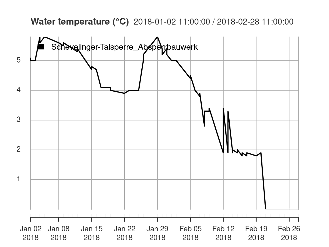
Let’s plot the received data as time series:
suppressPackageStartupMessages(library("xts"))
siteName = "Schevelinger-Talsperre_Absperrbauwerk"
dataColumn = 3
tsFluggs = xts(
  observationData[observationData$siteID == siteName, dataColumn],
  observationData[observationData$siteID == siteName, "timestamp"])
names(tsFluggs) = siteName
unitOfMeasurement = sosUOM(
  attributes(observationData[[dataColumn]])$defaultPointMetadata)
plot(x = tsFluggs,
     main = paste0("Water temperature (", unitOfMeasurement, ")"),
     sub = attributes(
       observationData[[dataColumn]]
       )$defaultPointMetadata@interpolationType@href,
     yaxis.right = FALSE, legend.loc = "topleft")
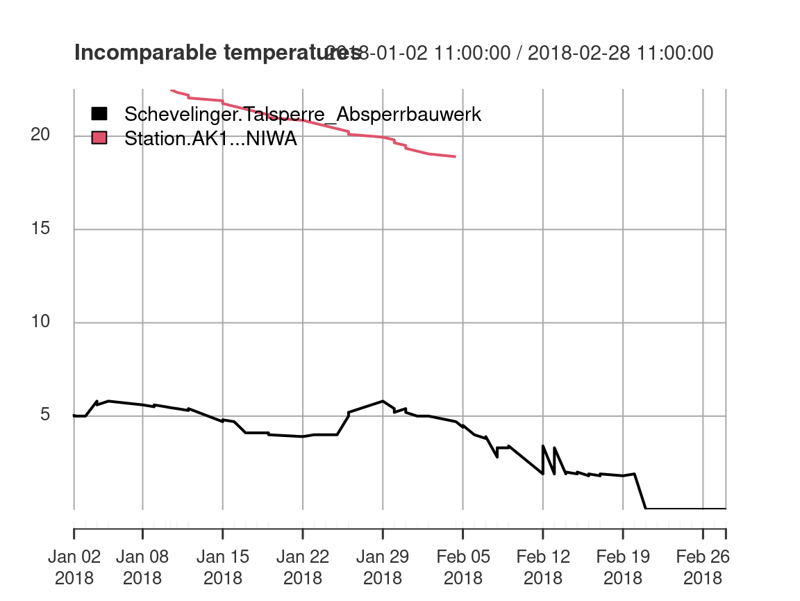
It is now straightforward to combine and visualize data from two different SOS servers. In this example, we’ll just combine water temperature from Germany and New Zealand.
niwa = SOS(
  url = "https://hydro-sos.niwa.co.nz/",
  binding = "KVP",
  useDCPs = FALSE,
  version = "2.0.0")
siteList = siteList(sos = niwa)
phenomenaNiwa = phenomena(sos = niwa)

observationDataNiwa = getData(sos = niwa,
  phenomena = phenomenaNiwa[25, 1],
  sites = siteList$siteID[40],
  begin = timeBegin,
  end = timeEnd)
attributes(observationDataNiwa[[3]])
## $metadata
## An object of class "WmlMeasurementTimeseriesMetadata"
## Slot "temporalExtent":
## GmlTimePeriod: [ GmlTimePosition [ time: 2018-01-10 21:15:00 ]
##  --> GmlTimePosition [ time: 2018-02-04 20:30:00 ] ]
##
##
## $defaultPointMetadata
## An object of class "WmlDefaultTVPMeasurementMetadata"
## Slot "uom":
## [1] "degC"
##
## Slot "interpolationType":
## An object of class "WmlInterpolationType"
## Slot "href":
## [1] "http://www.opengis.net/def/timeseriesType/WaterML/2.0/continuous"
##
## Slot "title":
## [1] "Instantaneous"

summary(observationDataNiwa)
##     siteID            timestamp                    Temperature
##  Length:2           Min.   :2018-01-10 21:15:00   Min.   :18.9
##  Class :character   1st Qu.:2018-01-17 03:03:45   1st Qu.:19.8
##  Mode  :character   Median :2018-01-23 08:52:30   Median :20.7
##                     Mean   :2018-01-23 08:52:30   Mean   :20.7
##                     3rd Qu.:2018-01-29 14:41:15   3rd Qu.:21.6
##                     Max.   :2018-02-04 20:30:00   Max.   :22.5
ts1056 = xts(observationDataNiwa[observationDataNiwa$siteID == 'AK1', 3],
             observationDataNiwa[observationDataNiwa$siteID == 'AK1',"timestamp"])
names(ts1056) = "Station#AK1 @ NIWA"
plot(
  x = na.fill(merge(tsFluggs, ts1056), list(NA, "extend", NA)),
  main = "Incomparable temperatures",
  yaxis.right = FALSE,
  legend.loc = 'topleft')
Shiny application
We also illustrate the use of the sos4R package in a simple, yet easily extensible Shiny web application. By default, the application queries a SOS service operated by the Wupperverband (see fluggs SOS above). This SOS provides various hydrological time series. Upon start-up, the app portrays all measurement stations reporting data in a given time window on a map (see screenshot below). The user can interactively change this time window in the sidebar on the left hand side of the user interface. After the user selects a single station on the map, a list with the phenomena available appears in the sidebar and the app downloads the data for the given period. The data retrieved is converted into an xts object and shown as a plot beneath the map window. The user can select one or more phenomena and the app will automatically update the plot with the newly retrieved data.
You can try out the app online at http://pilot.52north.org/shinyApps/sos4R/. The app’s source code, merely three function calls of sos4R wrapped in a simple graphical user interface, is part of the sos4R package.
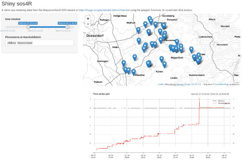
Shiny sos4R app screenshot
References
Nüst D., Stasch C., Pebesma E. (2011) Connecting R to the Sensor Web. In: Geertman S., Reinhardt W., Toppen F. (eds) Advancing Geoinformation Science for a Changing World. Lecture Notes in Geoinformation and Cartography, Springer. doi: 10.1007/978-3-642-19789-5_12
Pebesma, E., Nüst, D., & Bivand, R. (2012). The R software environment in reproducible geoscientific research. Eos, Transactions American Geophysical Union, 93(16), 163–163. doi: 10.1029/2012EO160003