Wrapper Functions for easier SOS access
Daniel Nüst , Eike Hinderk Jürrens, and Benedikt Gräler
Institute for Geoinformatics, University of Münster, Germany. 52°North GmbH, Münster, Germany.daniel.nuest@uni-muenster.de, e.h.juerrens@52north.org, and b.graeler@52north.org
2020-07-08
Source:vignettes/sos4R-vignette-05-wrapper-functions.Rmd
sos4R-vignette-05-wrapper-functions.RmdIntroduction
sos4R includes a collection of convenience functions which wrap the complex SOS interface with its specific terms (e.g. FOI, procedure). The wrapper function use more generic terms easily accessible for all users, especially without a strong knowledge of the OGC standards of the Sensor Web Enablement (see “OGC SWE and SOS” vignette for details).
In general, these functions always return an object of class data.frame, even if the result is only a list, in which case the data.frame has one column.
Shiny Demo App
A minimal Shiny app demonstrating the convenience functions is included in the package. Run it with
shiny::runApp(appDir = file.path(path.package("sos4R"), "shiny"))
Phenomena
The function phenomena(..) provides information about observed phenomena, time periods of data, and sites observing these phenomena.
phenomena <- phenomena(sos = mySos)
str(phenomena)
#> 'data.frame':    84 obs. of  1 variable:
#>  $ phenomenon: chr  "MTHLY_STATS: DAYS OF DEFICIT (WBal AWC=150mm) (MTHLY: DAYS OF DEFICIT (WBAL))" "MTHLY_STATS: DAYS OF OCCURRENCE (FOG) (MTHLY: FOG DAYS)" "MTHLY_STATS: DAYS OF OCCURRENCE (GALE) (MTHLY: GALE DAYS)" "MTHLY_STATS: DAYS OF OCCURRENCE (GROUND FROST) (MTHLY: GROUND FROST DAYS)" ...
phenomena[1:maxOutputRowsPerExample,]
#> [1] "MTHLY_STATS: DAYS OF DEFICIT (WBal AWC=150mm) (MTHLY: DAYS OF DEFICIT (WBAL))"
#> [2] "MTHLY_STATS: DAYS OF OCCURRENCE (FOG) (MTHLY: FOG DAYS)"
#> [3] "MTHLY_STATS: DAYS OF OCCURRENCE (GALE) (MTHLY: GALE DAYS)"
#> [4] "MTHLY_STATS: DAYS OF OCCURRENCE (GROUND FROST) (MTHLY: GROUND FROST DAYS)"
#> [5] "MTHLY_STATS: DAYS OF OCCURRENCE (GUSTS over 23 knots) (MTHLY: GUST DAYS 24)"
The retrieved data can be extended to the time intervals and site identifier for which data is available. The next example shows the overall temporal availability of the phenomena in the SOS instance:
phenomena(sos = mySos, includeTemporalBBox = TRUE)[1:maxOutputRowsPerExample,]
#>                                                                     phenomenon
#> 1                              MTHLY_STATS: TOTAL RAINFALL (MTHLY: TOTAL RAIN)
#> 2           MTHLY_STATS: WET DAYS with rainfall 1 mm or more (MTHLY: WET DAYS)
#> 3     MTHLY_STATS: MEAN AIR TEMPERATURE;   0.5* (MAX + MIN) (MTHLY: MEAN TEMP)
#> 4 MTHLY_STATS: MEAN MAXIMUM TEMPERATURE from daily Maxs (MTHLY: MEAN MAX TEMP)
#> 5 MTHLY_STATS: MEAN MINIMUM TEMPERATURE from daily Mins (MTHLY: MEAN MIN TEMP)
#>    timeBegin    timeEnd
#> 1 1960-08-01 2020-06-01
#> 2 1960-08-01 2020-06-01
#> 3 1960-08-01 2020-06-01
#> 4 1960-08-01 2020-06-01
#> 5 1960-08-01 2020-06-01
This example shows at which site the phenomena are available:
phenomena(sos = mySos, includeSiteId = TRUE)[1:maxOutputRowsPerExample,]
#>                                                                        phenomenon
#> 61  MTHLY_STATS: DAYS OF DEFICIT (WBal AWC=150mm) (MTHLY: DAYS OF DEFICIT (WBAL))
#> 126 MTHLY_STATS: DAYS OF DEFICIT (WBal AWC=150mm) (MTHLY: DAYS OF DEFICIT (WBAL))
#> 152 MTHLY_STATS: DAYS OF DEFICIT (WBal AWC=150mm) (MTHLY: DAYS OF DEFICIT (WBAL))
#> 251 MTHLY_STATS: DAYS OF DEFICIT (WBal AWC=150mm) (MTHLY: DAYS OF DEFICIT (WBAL))
#> 293 MTHLY_STATS: DAYS OF DEFICIT (WBal AWC=150mm) (MTHLY: DAYS OF DEFICIT (WBAL))
#>     siteID
#> 61   17244
#> 126  26958
#> 152  25506
#> 251  22719
#> 293  37850
You can also add both temporal extent and sites:
phenomena(sos = mySos, includeTemporalBBox = TRUE, includeSiteId = TRUE)[1:maxOutputRowsPerExample,]
#>                                                                        phenomenon
#> 61  MTHLY_STATS: DAYS OF DEFICIT (WBal AWC=150mm) (MTHLY: DAYS OF DEFICIT (WBAL))
#> 126 MTHLY_STATS: DAYS OF DEFICIT (WBal AWC=150mm) (MTHLY: DAYS OF DEFICIT (WBAL))
#> 152 MTHLY_STATS: DAYS OF DEFICIT (WBal AWC=150mm) (MTHLY: DAYS OF DEFICIT (WBAL))
#> 251 MTHLY_STATS: DAYS OF DEFICIT (WBal AWC=150mm) (MTHLY: DAYS OF DEFICIT (WBAL))
#> 293 MTHLY_STATS: DAYS OF DEFICIT (WBal AWC=150mm) (MTHLY: DAYS OF DEFICIT (WBAL))
#>     siteID  timeBegin    timeEnd
#> 61   17244 1999-08-01 2020-06-01
#> 126  26958 2007-08-01 2020-06-01
#> 152  25506 2004-12-01 2018-06-01
#> 251  22719 2002-07-01 2018-11-01
#> 293  37850 2011-11-01 2020-06-01
Sites With Coordinates
The function sites(..) provides information about sites where observations are performed, including metadata about the sites (e.g. location). The returned object is a SpatialPointsDataFrame.
sites <- sites(sos = mySos)
sites[1:maxOutputRowsPerExample,]
#>             coordinates siteID
#> 1    (173.926, -35.183)   1056
#> 2  (172.851, -42.53433)  11234
#> 3 (172.9716, -41.09798)  12429
#> 4 (173.9628, -41.49891)  12430
#> 5 (169.3148, -45.20724)  12431
To see all sites, even the ones without any data, use the empty parameter.
sites_with_empty <- sites(sos = mySos, empty = TRUE)
sites_with_empty[1:maxOutputRowsPerExample,]
#>             coordinates siteID empty
#> 1    (173.926, -35.183)   1056 FALSE
#> 2  (172.851, -42.53433)  11234 FALSE
#> 3 (172.9716, -41.09798)  12429 FALSE
#> 4 (173.9628, -41.49891)  12430 FALSE
#> 5 (169.3148, -45.20724)  12431 FALSE
You can retrieve additional metadata about the phenomena and the time period for which data is available. Including temporal extent implies inclusion of phenomena. In the next chunks the object is coerced to a date.frame to get a tabular view.
sites_with_phenomena <- sites(sos = mySos, includePhenomena = TRUE)
sites_with_phenomena[1:maxOutputRowsPerExample, 1:maxOutputColumnsPerExample]
#>             coordinates siteID
#> 1    (173.926, -35.183)   1056
#> 2  (172.851, -42.53433)  11234
#> 3 (172.9716, -41.09798)  12429
#> 4 (173.9628, -41.49891)  12430
#> 5 (169.3148, -45.20724)  12431
#>   MTHLY_STATS..DAYS.OF.DEFICIT..WBal.AWC.150mm...MTHLY..DAYS.OF.DEFICIT..WBAL..
#> 1                                                                          TRUE
#> 2                                                                          TRUE
#> 3                                                                          TRUE
#> 4                                                                          TRUE
#> 5                                                                          TRUE
#>   MTHLY_STATS..DAYS.OF.OCCURRENCE..FOG...MTHLY..FOG.DAYS.
#> 1                                                    TRUE
#> 2                                                   FALSE
#> 3                                                   FALSE
#> 4                                                   FALSE
#> 5                                                   FALSE
The next section show how to retrieve spatial information about the sites and temporal information about the available phenomena:
sites_with_temporal_bbox <- sites(sos = mySos, includePhenomena = TRUE, includeTemporalBBox = TRUE)
tail(sites_with_temporal_bbox, n = 3)[,1:maxOutputColumnsPerExample]
#>              coordinates siteID
#> 58 (171.8601, -42.11578)   3925
#> 59 (169.3182, -45.20342)  39564
#> 60  (169.6842, -45.0401)   5535
#>    MTHLY_STATS..DAYS.OF.DEFICIT..WBal.AWC.150mm...MTHLY..DAYS.OF.DEFICIT..WBAL..
#> 58                                                        -291945600, 1590969600
#> 59                                                        1333238400, 1590969600
#> 60                                                         539136000, 1590969600
#>    MTHLY_STATS..DAYS.OF.OCCURRENCE..FOG...MTHLY..FOG.DAYS.
#> 58                                   -297216000, 691545600
#> 59                                                      NA
#> 60                                                      NA
The following chunk shows how to get a better representation:
str(tail(sites_with_temporal_bbox, n = 3)[,1:maxOutputColumnsPerExample])
#> Formal class 'SpatialPointsDataFrame' [package "sp"] with 5 slots
#>   ..@ data       :'data.frame':  3 obs. of  3 variables:
#>   .. ..$ siteID                                                                       : chr [1:3] "3925" "39564" "5535"
#>   .. ..$ MTHLY_STATS: DAYS OF DEFICIT (WBal AWC=150mm) (MTHLY: DAYS OF DEFICIT (WBAL)):List of 3
#>   .. .. ..$ MTHLY_STATS: DAYS OF DEFICIT (WBal AWC=150mm) (MTHLY: DAYS OF DEFICIT (WBAL)):'data.frame':  1 obs. of  2 variables:
#>   .. .. .. ..$ timeBegin: POSIXct[1:1], format: "1960-10-01"
#>   .. .. .. ..$ timeEnd  : POSIXct[1:1], format: "2020-06-01"
#>   .. .. ..$ MTHLY_STATS: DAYS OF DEFICIT (WBal AWC=150mm) (MTHLY: DAYS OF DEFICIT (WBAL)):'data.frame':  1 obs. of  2 variables:
#>   .. .. .. ..$ timeBegin: POSIXct[1:1], format: "2012-04-01"
#>   .. .. .. ..$ timeEnd  : POSIXct[1:1], format: "2020-06-01"
#>   .. .. ..$ MTHLY_STATS: DAYS OF DEFICIT (WBal AWC=150mm) (MTHLY: DAYS OF DEFICIT (WBAL)):'data.frame':  1 obs. of  2 variables:
#>   .. .. .. ..$ timeBegin: POSIXct[1:1], format: "1987-02-01"
#>   .. .. .. ..$ timeEnd  : POSIXct[1:1], format: "2020-06-01"
#>   .. ..$ MTHLY_STATS: DAYS OF OCCURRENCE (FOG) (MTHLY: FOG DAYS)                      :List of 3
#>   .. .. ..$ MTHLY_STATS: DAYS OF OCCURRENCE (FOG) (MTHLY: FOG DAYS):'data.frame':    1 obs. of  2 variables:
#>   .. .. .. ..$ timeBegin: POSIXct[1:1], format: "1960-08-01"
#>   .. .. .. ..$ timeEnd  : POSIXct[1:1], format: "1991-12-01"
#>   .. .. ..$ MTHLY_STATS: DAYS OF OCCURRENCE (FOG) (MTHLY: FOG DAYS): logi NA
#>   .. .. ..$ MTHLY_STATS: DAYS OF OCCURRENCE (FOG) (MTHLY: FOG DAYS): logi NA
#>   ..@ coords.nrs : num(0)
#>   ..@ coords     : num [1:3, 1:2] 171.9 169.3 169.7 -42.1 -45.2 ...
#>   .. ..- attr(*, "dimnames")=List of 2
#>   .. .. ..$ : NULL
#>   .. .. ..$ : chr [1:2] "lon" "lat"
#>   ..@ bbox       : num [1:2, 1:2] 169.3 -45.2 171.9 -42.1
#>   .. ..- attr(*, "dimnames")=List of 2
#>   .. .. ..$ : chr [1:2] "lon" "lat"
#>   .. .. ..$ : chr [1:2] "min" "max"
#>   ..@ proj4string:Formal class 'CRS' [package "sp"] with 1 slot
#>   .. .. ..@ projargs: chr "+proj=longlat +datum=WGS84 +no_defs"
Filter Sites With Coordinates
You can filter sites using phenomena and temporal extent.
Note: When creating time objects from strings, as.POSIXct(..) by default recognises the local timezone and creates a time object in UTC.
sites_filtered_by_phenomena <- sites(sos = mySos, phenomena = phenomena[3,])
nrow(sites_filtered_by_phenomena@data)
#> [1] 60
str(sites_filtered_by_phenomena)
#> Formal class 'SpatialPointsDataFrame' [package "sp"] with 5 slots
#>   ..@ data       :'data.frame':  60 obs. of  1 variable:
#>   .. ..$ siteID: chr [1:60] "1056" "11234" "12429" "12430" ...
#>   ..@ coords.nrs : num(0)
#>   ..@ coords     : num [1:60, 1:2] 174 173 173 174 169 ...
#>   .. ..- attr(*, "dimnames")=List of 2
#>   .. .. ..$ : NULL
#>   .. .. ..$ : chr [1:2] "lon" "lat"
#>   ..@ bbox       : num [1:2, 1:2] -176.5 -77.8 177.9 -35.1
#>   .. ..- attr(*, "dimnames")=List of 2
#>   .. .. ..$ : chr [1:2] "lon" "lat"
#>   .. .. ..$ : chr [1:2] "min" "max"
#>   ..@ proj4string:Formal class 'CRS' [package "sp"] with 1 slot
#>   .. .. ..@ projargs: chr "+proj=longlat +datum=WGS84 +no_defs"
Use the parameter includeTemporalBBox for including additional metadata:
sites_filtered_by_phenomena_with_metadata <- sites(sos = mySos, phenomena = phenomena[3,], includePhenomena = TRUE, includeTemporalBBox = TRUE)
str(sites_filtered_by_phenomena_with_metadata)
#> Formal class 'SpatialPointsDataFrame' [package "sp"] with 5 slots
#>   ..@ data       :'data.frame':  2 obs. of  2 variables:
#>   .. ..$ siteID                                                   : chr [1:2] "1056" "3925"
#>   .. ..$ MTHLY_STATS: DAYS OF OCCURRENCE (GALE) (MTHLY: GALE DAYS):List of 2
#>   .. .. ..$ MTHLY_STATS: DAYS OF OCCURRENCE (GALE) (MTHLY: GALE DAYS):'data.frame':  1 obs. of  2 variables:
#>   .. .. .. ..$ timeBegin: POSIXct[1:1], format: "1981-10-01"
#>   .. .. .. ..$ timeEnd  : POSIXct[1:1], format: "1995-11-01"
#>   .. .. ..$ MTHLY_STATS: DAYS OF OCCURRENCE (GALE) (MTHLY: GALE DAYS):'data.frame':  1 obs. of  2 variables:
#>   .. .. .. ..$ timeBegin: POSIXct[1:1], format: "1960-08-01"
#>   .. .. .. ..$ timeEnd  : POSIXct[1:1], format: "1991-12-01"
#>   ..@ coords.nrs : num(0)
#>   ..@ coords     : num [1:2, 1:2] 173.9 171.9 -35.2 -42.1
#>   .. ..- attr(*, "dimnames")=List of 2
#>   .. .. ..$ : NULL
#>   .. .. ..$ : chr [1:2] "lon" "lat"
#>   ..@ bbox       : num [1:2, 1:2] 171.9 -42.1 173.9 -35.2
#>   .. ..- attr(*, "dimnames")=List of 2
#>   .. .. ..$ : chr [1:2] "lon" "lat"
#>   .. .. ..$ : chr [1:2] "min" "max"
#>   ..@ proj4string:Formal class 'CRS' [package "sp"] with 1 slot
#>   .. .. ..@ projargs: chr "+proj=longlat +datum=WGS84 +no_defs"
# under development - no github issue atm
#sites_filtered_by_time <- sites(sos = mySos, begin = parsedate::parse_iso_8601("1904-01-01"), end = parsedate::parse_iso_8601("1905-12-31"))
#nrow(sites_filtered_by_time@data)
#str(sites_filtered_by_time)
The SpatialPointsDataFrame allows access to coordinates with coordinate reference system (CRS).
sp::coordinates(sites)[1:maxOutputRowsPerExample,]
#>           lon       lat
#> [1,] 173.9260 -35.18300
#> [2,] 172.8510 -42.53433
#> [3,] 172.9717 -41.09798
#> [4,] 173.9629 -41.49891
#> [5,] 169.3148 -45.20724
sites@proj4string
#> CRS arguments: +proj=longlat +datum=WGS84 +no_defs
sp::bbox(sites)
#>            min       max
#> lon -176.47500 177.92180
#> lat  -77.84935 -35.13352
This object can be directly used as input for various mapping libraries, e.g. mapview.
suppressPackageStartupMessages(library("mapview"))

mapview(sites, legend = FALSE, col.regions = "blue")
Site Listings
The function siteList(..) provides information about observed phenomena at sites and the time periods when data is available.
siteList <- siteList(sos = mySos)
str(siteList)
#> 'data.frame':    60 obs. of  1 variable:
#>  $ siteID: chr  "1056" "11234" "12429" "12430" ...
You can extend the information returned with these parameters:
-
emptyto also show sites without data -
includePhenomenato add phenomena to the table (boolean) -
includeTemporalBBoxto also show the time when data is available (boolean)
siteList_with_empty <- siteList(sos = mySos, empty = TRUE)
siteList_with_empty[1:maxOutputRowsPerExample,]
#> [1] "1056"  "11234" "12429" "12430" "12431"
# under development - https://github.com/52North/sos4R/issues/90
#siteListe_with_metadata <- siteList(sos = mySos, includePhenomena = TRUE, includeTemporalBBox = TRUE)
#siteListe_with_metadata[1:maxOutputRowsPerExample,]
Filter Site Listings
You can filter the results with these parameters:
-
phenomenais a vector of phenomena which must be measured at the sites -
beginandenddefine a time interval (date and time class objects) for which some data must be available (sites may have data outside the given interval)
Note: When creating time objects from strings, as.POSIXct(..) by default recognises the local timezone and creates a time object in UTC.
siteList_filtered_by_time_and_phenomenon <- siteList(sos = mySos,
         phenomena = phenomena$phenomenon[1:2],
         begin = as.POSIXct("1950-01-01"), end = as.POSIXct("1960-12-31")
         )
siteList_filtered_by_time_and_phenomenon
#>   siteID
#> 1   3925
Data download
The function getData(..) retrieves the actual data and returns them in ready-to-use data structures from the spacetime package.
The returned data can be limited by thematical, spatial, and temporal filters. Thematical filtering (phenomena) support the values of the previous functions as inputs. Spatial filters are either sites, or a bounding box. Temporal filter is a time period during which observations are made.
Note: When creating time objects from strings, as.POSIXct(..) by default recognises the local timezone and creates a time object in UTC.
observationData <- getData(sos = mySos,
                           phenomena = phenomena[18,1],
                           sites = siteList[1,1],
                           begin = parsedate::parse_iso_8601("1970-01-01T12:00:00+12:00"),
                           end = parsedate::parse_iso_8601("2000-01-02T12:00:00+12:00")
                           )

str(observationData)
#> 'data.frame':    212 obs. of  3 variables:
#>  $ siteID                                                         : chr  "1056" "1056" "1056" "1056" ...
#>  $ timestamp                                                      : POSIXct, format: "1981-10-01" "1981-11-01" ...
#>  $ MTHLY_STATS: EXTREME MAXIMUM TEMPERATURE (MTHLY: EXTR MAX TEMP): num  20.6 21.9 25 27.8 29.2 24.5 22.9 20.7 18.3 18 ...
#>   ..- attr(*, "metadata")=Formal class 'WmlMeasurementTimeseriesMetadata' [package "sos4R"] with 1 slot
#>   .. .. ..@ temporalExtent:Formal class 'GmlTimePeriod' [package "sos4R"] with 9 slots
#>   .. .. .. .. ..@ begin        : NULL
#>   .. .. .. .. ..@ beginPosition:Formal class 'GmlTimePosition' [package "sos4R"] with 4 slots
#>   .. .. .. .. .. .. ..@ time                 : POSIXct[1:1], format: "1981-10-01"
#>   .. .. .. .. .. .. ..@ frame                : chr NA
#>   .. .. .. .. .. .. ..@ calendarEraName      : chr NA
#>   .. .. .. .. .. .. ..@ indeterminatePosition: chr NA
#>   .. .. .. .. ..@ end          : NULL
#>   .. .. .. .. ..@ endPosition  :Formal class 'GmlTimePosition' [package "sos4R"] with 4 slots
#>   .. .. .. .. .. .. ..@ time                 : POSIXct[1:1], format: "2000-01-01"
#>   .. .. .. .. .. .. ..@ frame                : chr NA
#>   .. .. .. .. .. .. ..@ calendarEraName      : chr NA
#>   .. .. .. .. .. .. ..@ indeterminatePosition: chr NA
#>   .. .. .. .. ..@ duration     : chr NA
#>   .. .. .. .. ..@ timeInterval : NULL
#>   .. .. .. .. ..@ frame        : chr NA
#>   .. .. .. .. ..@ relatedTimes : list()
#>   .. .. .. .. ..@ id           : chr "phenomenonTime_1"
#>   ..- attr(*, "defaultPointMetadata")=Formal class 'WmlDefaultTVPMeasurementMetadata' [package "sos4R"] with 2 slots
#>   .. .. ..@ uom              : chr "DEGREE_CELSIUS"
#>   .. .. ..@ interpolationType:Formal class 'WmlInterpolationType' [package "sos4R"] with 2 slots
#>   .. .. .. .. ..@ href : chr "http://www.opengis.net/def/timeseriesType/WaterML/2.0/continuous"
#>   .. .. .. .. ..@ title: chr "Instantaneous"
Get an overview of the data using the summary function:
summary(observationData)
#>     siteID            timestamp
#>  Length:212         Min.   :1981-10-01 00:00:00
#>  Class :character   1st Qu.:1986-02-22 00:00:00
#>  Mode  :character   Median :1990-07-16 12:00:00
#>                     Mean   :1990-09-03 15:50:56
#>                     3rd Qu.:1995-02-08 00:00:00
#>                     Max.   :2000-01-01 00:00:00
#>  MTHLY_STATS: EXTREME MAXIMUM TEMPERATURE (MTHLY: EXTR MAX TEMP)
#>  Min.   :17.10
#>  1st Qu.:20.10
#>  Median :22.95
#>  Mean   :23.24
#>  3rd Qu.:26.20
#>  Max.   :30.20
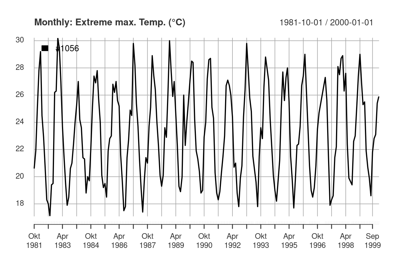
Timeseries Plotting
Plot received data as time series:
suppressPackageStartupMessages(library(xts))
ts1056 <- xts(observationData[observationData$siteID == '1056',3], observationData[observationData$siteID == '1056',"timestamp"])
names(ts1056) <- "#1056"
plot(x = ts1056, main = "Monthly: Extreme max. Temp. (°C)", yaxis.right = FALSE, legend.loc = 'topleft')
The next example gets data for two phenomena a site.
# TO BE IMPLEMENTED: merge different observation types - see https://github.com/52North/sos4R/issues/96#issuecomment-493424151
observationData <- getData(sos = mySos,
       phenomena = phenomena$phenomenon[1:2],
       sites = siteList$siteID[c(1,58)],
       begin = parsedate::parse_iso_8601("1994-12-31T12:00:00+12:00"),
       end = parsedate::parse_iso_8601("1995-12-31T12:00:00+12:00")
       )
str(observationData)
#> 'data.frame':    23 obs. of  4 variables:
#>  $ siteID                                                                       : Factor w/ 2 levels "1056","3925": 1 1 1 1 1 1 1 1 1 1 ...
#>  $ timestamp                                                                    : POSIXct, format: "1995-01-01" "1995-02-01" ...
#>  $ MTHLY_STATS: DAYS OF DEFICIT (WBal AWC=150mm) (MTHLY: DAYS OF DEFICIT (WBAL)): num  9 9 0 0 0 0 0 0 0 0 ...
#>   ..- attr(*, "metadata")=Formal class 'WmlMeasurementTimeseriesMetadata' [package "sos4R"] with 1 slot
#>   .. .. ..@ temporalExtent:Formal class 'GmlTimePeriod' [package "sos4R"] with 9 slots
#>   .. .. .. .. ..@ begin        : NULL
#>   .. .. .. .. ..@ beginPosition:Formal class 'GmlTimePosition' [package "sos4R"] with 4 slots
#>   .. .. .. .. .. .. ..@ time                 : POSIXct[1:1], format: "1995-01-01"
#>   .. .. .. .. .. .. ..@ frame                : chr NA
#>   .. .. .. .. .. .. ..@ calendarEraName      : chr NA
#>   .. .. .. .. .. .. ..@ indeterminatePosition: chr NA
#>   .. .. .. .. ..@ end          : NULL
#>   .. .. .. .. ..@ endPosition  :Formal class 'GmlTimePosition' [package "sos4R"] with 4 slots
#>   .. .. .. .. .. .. ..@ time                 : POSIXct[1:1], format: "1995-12-01"
#>   .. .. .. .. .. .. ..@ frame                : chr NA
#>   .. .. .. .. .. .. ..@ calendarEraName      : chr NA
#>   .. .. .. .. .. .. ..@ indeterminatePosition: chr NA
#>   .. .. .. .. ..@ duration     : chr NA
#>   .. .. .. .. ..@ timeInterval : NULL
#>   .. .. .. .. ..@ frame        : chr NA
#>   .. .. .. .. ..@ relatedTimes : list()
#>   .. .. .. .. ..@ id           : chr "phenomenonTime_1"
#>   ..- attr(*, "defaultPointMetadata")=Formal class 'WmlDefaultTVPMeasurementMetadata' [package "sos4R"] with 2 slots
#>   .. .. ..@ uom              : chr "DAY"
#>   .. .. ..@ interpolationType:Formal class 'WmlInterpolationType' [package "sos4R"] with 2 slots
#>   .. .. .. .. ..@ href : chr "http://www.opengis.net/def/timeseriesType/WaterML/2.0/continuous"
#>   .. .. .. .. ..@ title: chr "Instantaneous"
#>  $ MTHLY_STATS: DAYS OF OCCURRENCE (FOG) (MTHLY: FOG DAYS)                      : num  1 0 0 5 4 2 3 1 0 0 ...
#>   ..- attr(*, "metadata")=Formal class 'WmlMeasurementTimeseriesMetadata' [package "sos4R"] with 1 slot
#>   .. .. ..@ temporalExtent:Formal class 'GmlTimePeriod' [package "sos4R"] with 9 slots
#>   .. .. .. .. ..@ begin        : NULL
#>   .. .. .. .. ..@ beginPosition:Formal class 'GmlTimePosition' [package "sos4R"] with 4 slots
#>   .. .. .. .. .. .. ..@ time                 : POSIXct[1:1], format: "1995-01-01"
#>   .. .. .. .. .. .. ..@ frame                : chr NA
#>   .. .. .. .. .. .. ..@ calendarEraName      : chr NA
#>   .. .. .. .. .. .. ..@ indeterminatePosition: chr NA
#>   .. .. .. .. ..@ end          : NULL
#>   .. .. .. .. ..@ endPosition  :Formal class 'GmlTimePosition' [package "sos4R"] with 4 slots
#>   .. .. .. .. .. .. ..@ time                 : POSIXct[1:1], format: "1995-11-01"
#>   .. .. .. .. .. .. ..@ frame                : chr NA
#>   .. .. .. .. .. .. ..@ calendarEraName      : chr NA
#>   .. .. .. .. .. .. ..@ indeterminatePosition: chr NA
#>   .. .. .. .. ..@ duration     : chr NA
#>   .. .. .. .. ..@ timeInterval : NULL
#>   .. .. .. .. ..@ frame        : chr NA
#>   .. .. .. .. ..@ relatedTimes : list()
#>   .. .. .. .. ..@ id           : chr "phenomenonTime_2"
#>   ..- attr(*, "defaultPointMetadata")=Formal class 'WmlDefaultTVPMeasurementMetadata' [package "sos4R"] with 2 slots
#>   .. .. ..@ uom              : chr "DAY"
#>   .. .. ..@ interpolationType:Formal class 'WmlInterpolationType' [package "sos4R"] with 2 slots
#>   .. .. .. .. ..@ href : chr "http://www.opengis.net/def/timeseriesType/WaterML/2.0/continuous"
#>   .. .. .. .. ..@ title: chr "Instantaneous"
You can also retrieve data for phenomena from multiple sites.
multipleSites <- siteList$siteID[1:2]
observationData <- getData(sos = mySos,
                           phenomena = phenomena[18, 1],
                           sites = multipleSites,
                           begin = parsedate::parse_iso_8601("1997-01-01T12:00:00+12:00"),
                           end = parsedate::parse_iso_8601("2000-01-02T12:00:00+12:00")
                           )


ts1056 <- xts(observationData[observationData$siteID == '1056', 3], observationData[observationData$siteID == '1056',"timestamp"])
names(ts1056) <- "Station#1056"
ts11234 <- xts(observationData[observationData$siteID == '11234', 3], observationData[observationData$siteID == '11234',"timestamp"])
names(ts11234) <- "Station#11234"
plot(x = na.fill(merge(ts1056, ts11234), list(NA, "extend", NA)), main = "Monthly: Extreme max. Temp. (°C)", yaxis.right = FALSE, legend.loc = 'topleft')
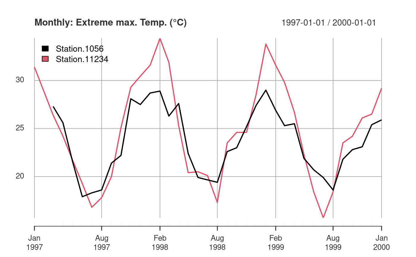
Map of the according sites:
sites_of_timeseries <- sites[sites$siteID == "1056" | sites$siteID == "11234",]
mapview(sites_of_timeseries, legend = FALSE, col.regions = "blue")