Isofuel Algorithm
General concept
The routing process is divided into individual routing steps. For every step, the distance is calculated that the ship can travel following different courses with a specified amount of fuel and constant speed. Only those routes that maximise the travel distance for a constant amount of fuel are selected for the next routing step. This optimisation process is referred to as pruning. The distance between the start coordinates at the beginning of the routing step and the end coordinates after the step is referred to as route segment.
The algorithm is the following:
Define the amount of fuel \(f_{max}\) that the ship can consume for every single routing step.
Consider a selection of courses outgoing from the start coordinate pair. For every course, calculate the fuel rate f/t (the amount of fuel consumed per time interval) that is necessary to keep the ship speed and course.
Based on \(f/t\), \(f_{max}\) and the ship speed, calculate the distance that is traveled for every route segment.
Divide the angular region into equally-sized segments – the pruning segments. For every pruning segment, the end point of the route segment that maximises the distance is passed as a new starting point to the next routing step.
Repeat steps 2. to 4. until the distance of any route from the starting coordinates towards the destination is smaller than the length of the route segment from the current routing step.
Obviously, the amount of fuel \(f_{max}\) that is provided to the algorithm determines the step width of the final route: the larger \(f_{max}\), the longer the route segments and the more edgy the final route. The number \(n_{courses}\) of courses that is considered for every coordinate pair defines the resolution with which the area is searched for optimal routes. Thus, the smaller \(n_{courses}\), the larger the likelihood that more optimal routes exist than the final route provided. On the other hand, the larger \(n_{courses}\) the larger is the calculation power. Further settings that can be defined are the area that is considered for the pruning as well as the number \(n_{prune}\) of pruning segments. The later specifies the number of end points that are passed from one routing step to the next. The relation of \(n_{courses}\) and \(n_{prune}\) defines the degree of optimisation.
Parameter and variable definitions
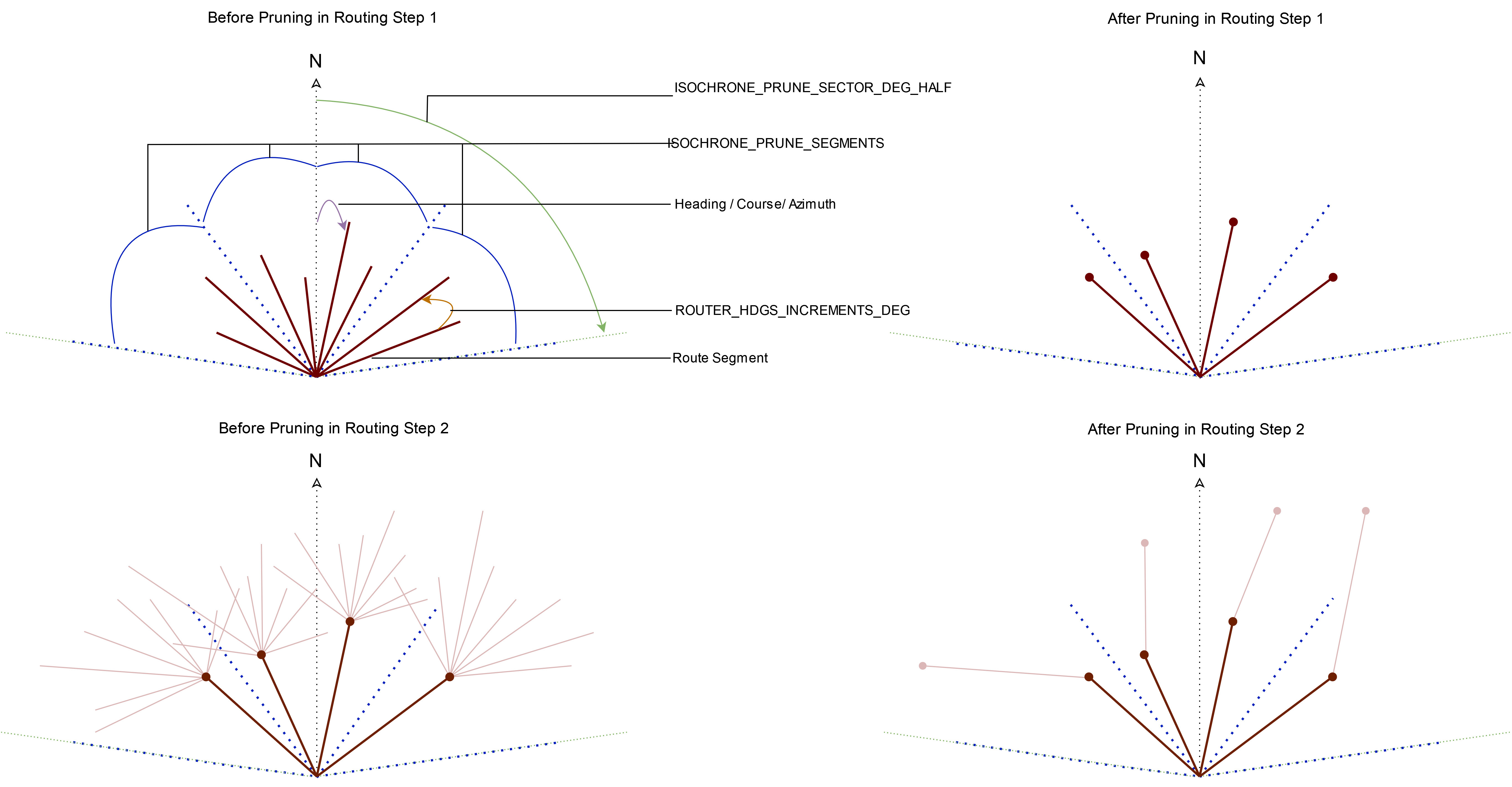
Fig.2: Schema for the definition of the most important parameter names for the isofuel algorithm.
ISOCHRONE_PRUNE_SEGMENTS = number of segments that are used for the pruning processISOCHRONE_PRUNE_SECTOR_DEG_HALF = angular range of azimuth angle that is considered for pruning (only one half of it!)ROUTER_HDGS_SEGMENTS = total number of courses/azimuths/headings that are considered per coordinate pair for every routing stepROUTER_HDGS_INCREMENTS_DEG = angular distance between two adjacent routing segmentsheading/course/azimuth/variants = the angular distance towards North on the grand circle routelats_per_step: (M,N) array of latitudes for different routes (shape N=headings+1) and routing steps (shape M=steps,decreasing)lons_per_step: (M,N) array of longitude for different routes (shape N=headings+1) and routing steps (shape M=steps,decreasing)Pruning methods
The pruning is the basis of the optimisation process for the isofuel algorithm. There exist three major concepts that can be used to adjust the pruning:
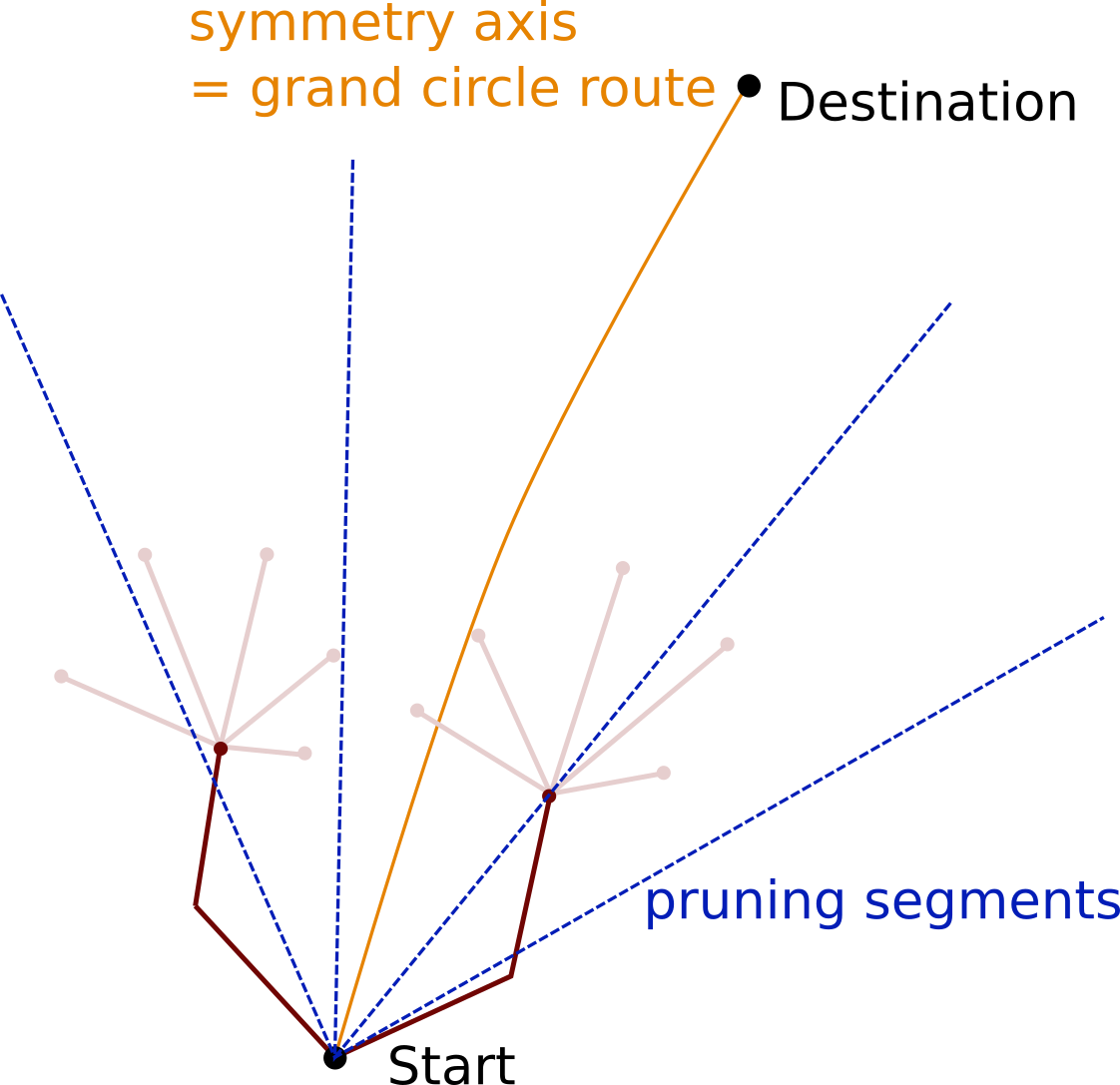
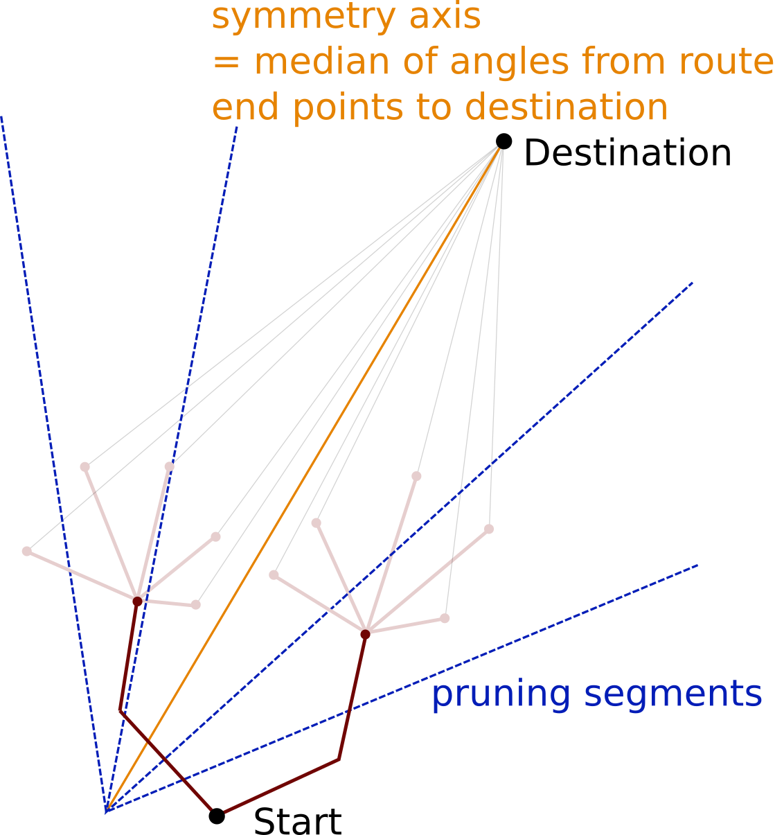
The definition of the angular region that is used for the pruning. This is specified by the number of pruning segments, the reach of the pruning sector and, most importantly, the angle around which the pruning segments are centered – in the following refered to as symmetry axis
The choice of how route segments are grouped for the pruning.
The optimisation criterion that is used as basis for the pruning.
The Definition of the Symmetry Axis
Two methods for the definition of the symmetry axis can be selected:
The symmetry axis is defined by the grand circle distance between the start point and the destination. In case intermediate waypoints have been defined, the intermediate start and end point are utilised.
The symmetry axis is defined by the median of the angles with respect to North of the connecting lines between the end of the route segments and the destination.
Grouping Route Segments
Route segments are organised in groups before the pruning is performed. Segments that lie outside of the pruning sector (shaded pink area in figures below) are exclueded from the pruning (dashed grey lines). The segment of one group that performs best regarding the minimisation criterion, survives the pruning process (solid pink lines). Three possibilities are available for grouping the route segments for the pruning:
courses-based: Route segments are grouped according to their courses.
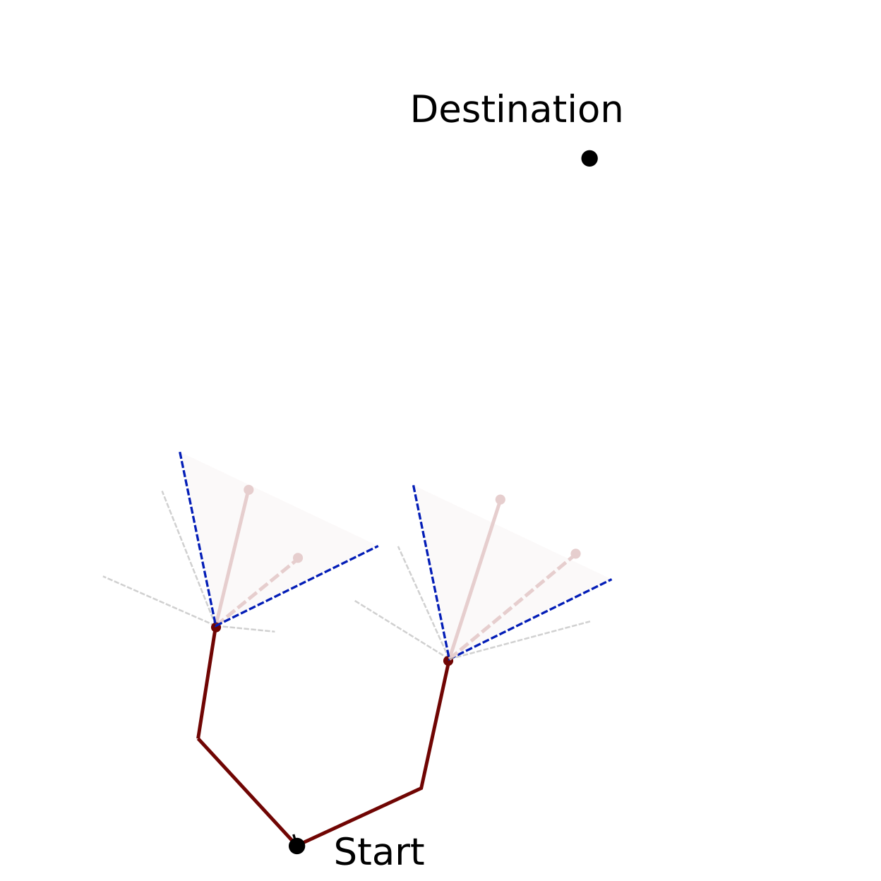
larger-direction-based: Route segments are grouped accoding to the angle of the connecting line between the global start point and the end of the route segment.
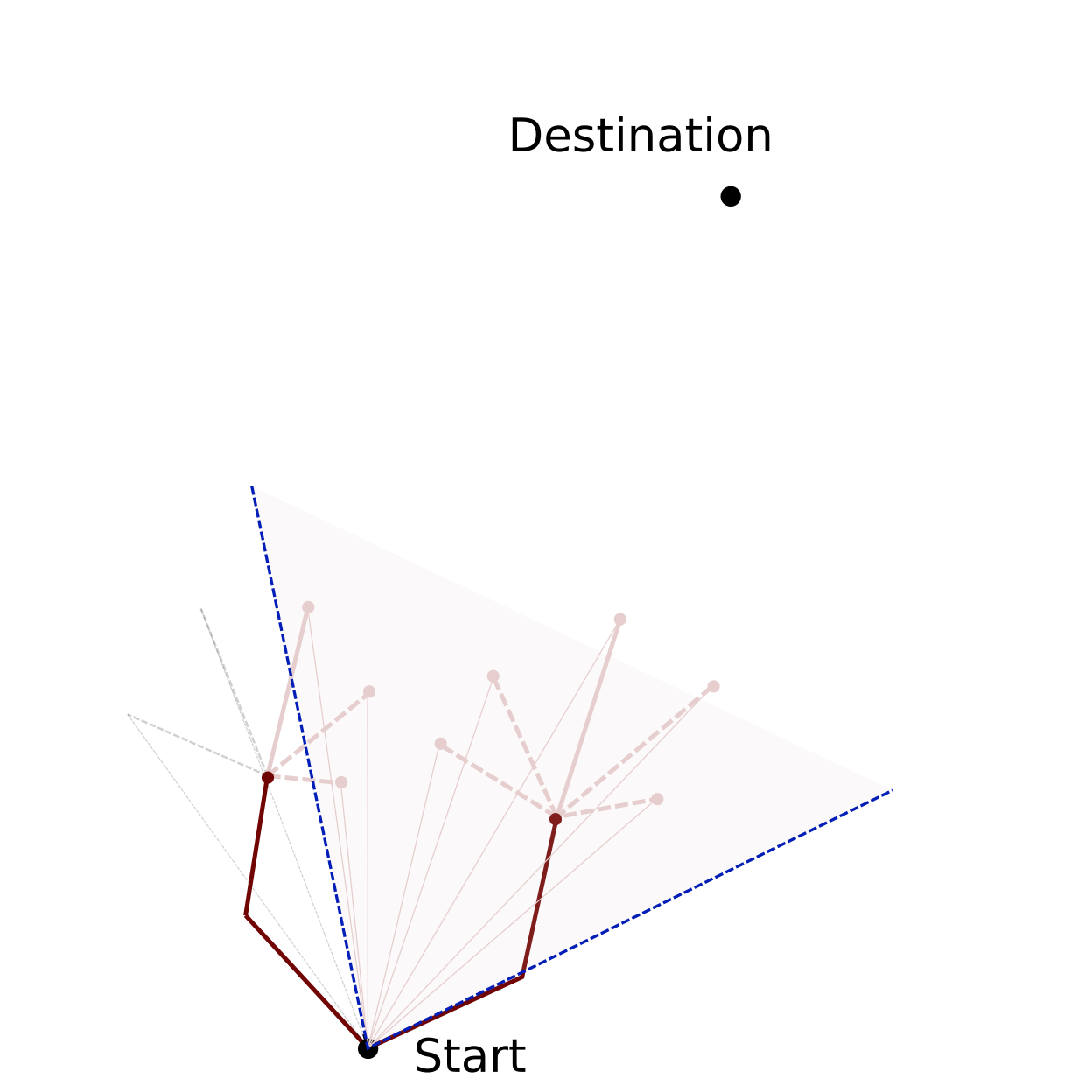
branch-based: Route segments of one branch form a group. Thus all route segments are considered for the pruning. For a particular routing step, a branch is the entity of route segments that originate from one common point.
The Optimisation Criterion
The optimisation criterion is the route property based on which routes are selected for the next routing step, i.e. the route property that is optimised. The Isofuel algorithm can be configured with one out of two optimisation criteria:
ISOCHRONE_MINIMISATION_CRITERION=”squareddist_over_disttodest”: the square of the total travel distance of the route at the current waypoint over the distance towards the destination
ISOCHRONE_MINIMISATION_CRITERION=”dist”: the total travel distance of the route
The optimisation criterion 1. has be chosen as default setting as for criterion 2., routes do not experience a drag towards the destination and tend to get lost in complex scenarios.